
Give yourself a pat on the back if you’ve come this far. You have used simple exact solutions to differential equations to grasp the essentials of non-equilibrium processes. But there’s the physical process on the one hand, and the mathematical description on the other. We’ve used continuous-time math thus far. We now move to discrete time and get a taste for “Markov state models,” which implicitly employ time discretization in the field of biomolecular simulation.
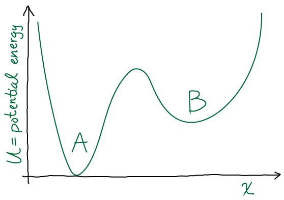
Let’s first review the questions from last time, based on the following pictures.
-
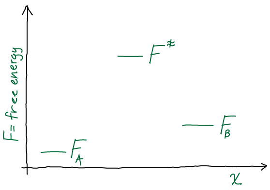
Draw a discrete free energy-level diagram corresponding to the continuous two state (A,B) system sketched above. Your diagram should consist of three free energy levels (A, B, barrier). Write down the Arrhenius expressions (in which the rate constant is proportional to the Boltzmann factor of the free-energy barrier height) in both directions. If the conformational free energy
 is defined according to
  , show that using Arrhenius-like rate constants causes detailed-balance to be satisfied.
-
In the Arrhenius picture, the rate constant for a transition is given by the product of a prefactor
 , which can be considered an attempt frequency, and a Boltzmann factor of the barrier height, which can be considered the probability of success. One ambiguity is whether the Boltzmann factor should be given in terms of the potential or free energy. We shall see that the free energy makes the estimate more reasonable and convenient, but note that the whole formulation is somewhat ad hoc and non-rigorous. We have
![\[k_{AB} = k_0 \, e^{-(F^\ddagger - F_A)/k_B T} \hspace{1cm} k_{BA} = k_0 \, e^{-(F^\ddagger - F_B)/k_B T}.\]](https://statisticalbiophysicsblog.org/wp-content/ql-cache/quicklatex.com-93535702821f885e7adf91090433d829_l3.png "Rendered by QuickLaTeX.com")
Having used the same prefactor
for both rates leads to the satisfaction of detailed balance based on the equilibrium Boltzmann factor given above,  , where the unknown constant
  is the same for both A and B. Detailed balance is confirmed by simple multiplication:
 ![\[P^{eq}_A k_{AB} = C k_0 e^{-F^\ddagger/k_B T} = P^{eq}_B k_{BA}\]](https://statisticalbiophysicsblog.org/wp-content/ql-cache/quicklatex.com-901f5ab3e31f0b548daef53c9ccf9f5c_l3.png "Rendered by QuickLaTeX.com")
-
In the Arrhenius picture, the rate constant for a transition is given by the product of a prefactor
-
What reasonable explanation can be given for the Arrhenius rate expression in terms of continuous-space equilibrium-ish statistical mechanics? And why should entropy differences enter the expression based on a one-dimensional picture?
-
The dimensionless Boltzmann factor of the free energy difference (between barrier top and initial state) represents a relative equilibrium probability. In the context of a non-equilibrium transition, a hand-waving explanation is that this dimensionless probability represents the chances to surmount the barrier given a constant attempt frequency . Entropy enters the free energy of the initial state in the standard way, so that larger entropy means lower free energy and hence lower success probability. The intuition is that entropy for a single state characterizes the effective width of that state, so a wider state means a trajectory will reach the edge less often and effectively have a lower attempt frequency. Of course, we have assumed the attempt frequency is constant, so the entropy of the initial state can be said to correct this frequency.
-
The dimensionless Boltzmann factor of the free energy difference (between barrier top and initial state) represents a relative equilibrium probability. In the context of a non-equilibrium transition, a hand-waving explanation is that this dimensionless probability represents the chances to surmount the barrier given a constant attempt frequency
-
Describe a procedure by which you could computationally estimate the rate constants of a continuous two-state system by running trajectories.
- We could simply start many trajectories in state A and run molecular dynamics until each reaches B. From that data, we could calculate the mean first-passage time (MFPT) and estimate the rate as 1/MFPT. Or we could calculate correlation functions from the simulated trajectories and use them to estimate rates.
It’s finally time to connect our knowledge of continuous-time systems to discrete-time dynamical descriptions of discrete states, known as “Markov state models.” That is, how do Markov state models arise from continuous descriptions? We have just made (above) a crude connection between continuous potentials and discrete states, and this will suffice for now. So we will implicitly assume our discrete states are single deep energy basins that indeed behave in a Markovian fashion – i.e., the probability of transitions out of the state do not depend on the path taken to get to the state. Note that this is very special property and one you should not generally expect to be satisfied in a tractable way for an atomically accurate description of a complex system – though this is a topic for another day.
The following questions build directly on notes you have already been studying. We will adopt the somewhat annoying notation that  refers to the
  transition probability. There’s a technical reason for this if you want to deal with the matrices, but at least I want to be consistent with my prior notes.
-
Give the full definition of
 and explain why it’s dimensionless.
 -
If
 is the time-dependent probability of state
  , show that
  .
. -
Using the exact solutions to the continuous-time two-state probabilities,
 , which we derived previously, calculate the discrete-time transition probabilities
  and
and  for transitions into state A. This problem is trickier than it sounds (though the math is easy), but don’t worry the derivation is there for you in the notes. The key trick is to write
  in terms of
  and
and  using the fact that
  for any/all
  .
.