

When we want to estimate parameters from data (e.g., from binding, kinetics, or electrophysiology experiments), there are two tasks: (i) estimate the most likely values, and (ii) equally importantly, estimate the uncertainty in those values. After all, if the uncertainty is huge, it’s hard to say we really know the parameters. We also need to choose the model in the first place, which is an extremely important task, but that is beyond the scope of this discussion.
While maximum likelihood (ML) estimates are clearly a sensible choice for parameter values, sometimes the ML approach is extended to provide confidence intervals, i.e., uncertainty ranges. In this discussion, I will explain why ML can be problematic for uncertainty in parameter values. As I have seen it applied (see Further Reading, below), ML is an approximation that is formally equivalent to a physical description of a system that ignores entropy. To be clear, ignoring entropy in a probabilistic sense is intrinsic to ML, and has nothing to do with whether entropy is being considered among physical parameters for data analysis. More on this below.
I believe that using ML is not a good idea for uncertainty, even though it may work ‘well enough’ in some cases. A key limitation is that the ML approach on its own cannot reveal when its approximation is a reasonable one.
Before getting into the critique, I will say that the right approach is Bayesian inference (BI). If you find BI confusing, let’s make clear at the outset that BI is simply a combination of likelihood – the very same ingredient that’s in ML already – and prior assumptions, which often are merely common-sense and/or empirical limits on parameter ranges … and such limits may be in place for ML estimates too. So don’t be afraid of BI theory … it’s quite similar to ML until the approximations come in. In fact, subtleties that enter prior selection in BI actually are implicit in ML approaches – see below.
You may know that BI calculations tend to be more computationally demanding than ML and certainly can be trickier. But I would say that in cases where the parameter likelihood or error landscape (defined below) is simple – both ML and BI will be straightforward. In cases where that landscape is challenging, both ML and BI will require care. In my opinion, typical BI practices are more likely to reveal a challenging landscape. But anyway, even in a simple landscape ML has the missing-entropy approximation problem.
Into the weeds: Words and pictures
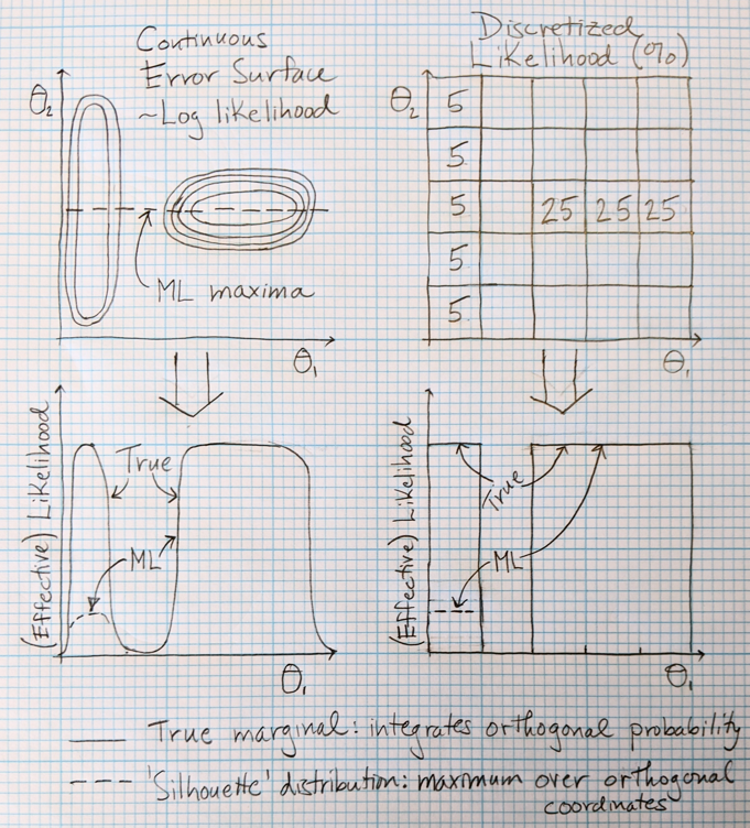
Before writing down any equations, let’s make clear the conceptual error that occurs with ML uncertainty estimation (as I have seen it practiced). The error comes from restricting attention to the subset of maximum likelihood solutions in a multi-dimensional space instead of considering all likelihood. In the simplest non-trivial case with two parameters  and
and  (see figure), the ML estimate of uncertainty for considers only the set of values that maximize the likelihood for each value of . That is, for each , the ML analysis considers only a single
  value which maximizes likelihood for the given . This ignores that the likelihood of any is determined not only by this maximum but by all possible values. In more technical terms, the likelihood associated with each is determined by the well-known marginal distribution, not by what might be dubbed the ‘silhouette’ distribution based only on the maxima (see figure). The ML approach ignores potentially significant variability that may occur in orthogonal variables ( in the simple example), and such variability is expected whenever there are non-linear correlations.
In statistical mechanics, the ML approximation is equivalent to generating a free energy surface that ignores entropy – i.e., is determined only by the lowest-energy configuration at each value of the coordinate(s) considered. (See Zuckerman textbook.) For complex systems not at low temperatures, such an approximation would not generally be reliable.
There’s no question that the ML approach just outlined is not correct and must be viewed as an approximation. The only rigorous way to check the approximation that I can see is to consider the full likelihood distribution … which is just Bayesian inference. In other words, it seems that we need to do BI to check if the ML approximation is ok.
Into the weeds: Equations
Let’s dive into the math, which fortunately isn’t too terrible. On the one hand, you have your data, which we’ll denote as  values. On the other, you have a mathematical model with some unknown parameters
  that are to be compared to the data: the model leads to predicted
  that depend on the specific set of parameters.
The difference between the data and the model can be quantified for any given set of parameters by examining a quantity related to the sum of squared deviations, given in the simplest case by
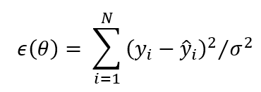
where  is the number of data points with values and where are the values generated by the model (for any given choice of parameters:
  ) and
) and  is the noise variance, which is often considered a separate (‘nuisance’) parameter. We will consider
  to be a vector listing the full set of parameters. In one case of particular interest to us, isothermal titration (ITC) calorimetry for simple binding, we have
  .
.
How do we get our ‘fitted’ parameters and uncertainties? In the absence of usable prior information, the Bayesian and Maximum Likelihood pictures agree that the most likely set of parameters is the one that minimizes the squared error function  . The agreement between the two approaches stems from the common (sense) view that the probability that a given set of parameters decreases as error increases. In fact, this is often made explicit through a Gaussian noise assumption which leads to a simple equation for the likelihood
  (i.e., probability – not normalized for simplicity) of a set of parameters as
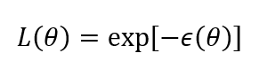
We can assume this equation is exact for the purposes of our discussion. A different form of the likelihood function doesn’t change the conclusions we’ll reach.
Let’s think about the ‘space’ of parameters, which is a fancy way of saying we’ll consider all possible sets of parameters, e.g.,  in the (simplified) ITC case. We can consider this space in the context of error
  or likelihood – which give the same information because one is the negative log of the other. In particular, think of what might be termed an ‘error surface’, a schematic of which is sketched in two dimensions
  in the figure so we can visualize it.
This error surface/probability distribution/energy landscape shows how using a ML strategy on a subset of variables ( in this case) artifactually shifts probability in the space. By taking only the most probable value of for each value, we discard some – potentially most – of the information contained in the coordinate. This approximation is equivalent to looking at a silhouette of the joint distribution (looking in the direction), rather than integrating (summing) over all pertinent values of . Mathematically, the ML approach amounts to considering  , i.e., for each we consider only the value which maximizes the likelihood.
Generically, the ML approach will lead to errors in predicted confidence intervals. Formulating this in mathematical language, the true probabilistic marginal which integrates (sums) over all probability is not the same as the (implied) ML distribution, i.e., the silhouette distribution:

Here, “Normalized{ … }” simply means the function in braces is normalized to a probability of 1 so we are making an apples-to-apples fair comparison. The left side represents the true marginal – used in BI –which includes all probability consistent with each value (integrated over ) whereas the right side is the “silhouette” distribution implicit in the ML approach which reflects only a single for each . Equality is not expected in general, though it will hold exactly for uncorrelated variables, and I would expect it to hold approximately for linearly correlated variables. If the two normalized probability densities are not the same, confidence intervals computed from them will generally differ.
In a statistical mechanics sense, the error function is analogous to the energy, so the error surface is like an energy landscape. The scaled noise variance  is analogous to the temperature: with less noise or more data, the distribution will become narrower. Ignoring all energy values except the minimum is equivalent to ignoring entropy.
In the equation above, the variables and can be considered vectors when considering the case of more than two dimensions. Although I do not know of a rigorous result regarding higher dimensions, my intuition is that ignoring more dimensions in a higher dimensional problem will increase the severity of the error in the ML approximation.
From my perspective, why would you use an approximation when there is a correct approach available?
Regarding the estimation of other features of the distribution, the ML process will likewise lead to approximation. This applies, for example, to the correlation structure, which fits into the formulation above: say we want to understand correlations among two parameters  which may be considered as a vector for the equations above. In exact analogy to the two-parameter description, we can contrast integrating over all other parameters
  in a BI picture vs. maximizing over those additional parameters. From these different mathematical operations, we expect different results – though the nature of the difference will depend on the precise joint parameter distribution of the system … which is unknown in advance.
Practical considerations in Bayesian vs. Maximum Likelihood error estimation
There’s no doubt that Bayesian computations require care and expertise – though we and others are working to reduce that burden. On the other hand, based on some experience, I believe that ML calculations require more care than some practitioners may realize – potentially compounding the approximation noted above with numerical errors. The problem for ML is that in a challenging system where the error landscape is not smooth, the well-known problem of start-point bias may corrupt the maximization process. That is, different starting values for parameters in the maximization may lead to different apparent ML values, and this won’t be detected unless the practitioner is extremely careful … and even if detected may be challenging to fix. (This issue is independent of the missing entropy, which can’t be fixed in ML.)
Bayesian inference, by contrast, attempts to sample the likelihood landscape – all of it that contributes appreciably to the likelihood. This requires a different mindset, but I would say a better awareness of the full space. BI also requires more computing, but to my mind this is completely worthwhile. After all, experimentalists may spend weeks or months preparing samples, calibrating equipment, and gathering data, so what’s the big deal about spending a few hours or days to analyze it?
A more speculative point about using BI is my belief that it promotes “landscape awareness.” That is, serious BI will involve critical examination of sampling – hopefully through replicate sampling runs – that forces the user to reckon with challenges in the system. A sampling mindset in which one worries about sampling quality/replicability is extremely valuable for obtaining reliable results.
I will note that some very complex systems may be out of reach for current BI software, but sampling checks should reveal whether this is the case, and then ML can be attempted. On the other hand, if you do sample the landscape well under BI, you can also extract ML values, but without the start-point bias noted above. I would also point out that BI developers are working actively to make software that is more powerful and reliable.
A word about priors: they’re not just for Bayesian inference
Prior assumptions and knowledge are part of doing science, and the quantification of such information is always a part of doing parameter uncertainty analysis whether we realize it or not. That is, the ‘prior’ (assumed distribution of possible outcomes in the absence of data) is an implicit part of maximum likelihood and Bayesian uncertainty quantification.
In the simplest case, we may assume a range of possible values for a given parameter. We hope that the likelihood function becomes negligible near the limits of our assumed range, and then we may imagine the prior had no bearing on our uncertainty range. This is not quite true, either for BI or ML.
The complication for both BI and ML is that typically there is no unique, fundamental representation of a parameter. In ITC analysis, for example, we are interested in binding free energies  but these can often be expressed in terms of the dissociation constant
  . In a different system, we might be interested in an angle measured in degrees, but we also might describe it via the cosine of the angle. Those familiar with Jacobians will recognize the problem: our representation of the parameter will affect how much probability is allotted to different parts of the parameter range of interest. Consider the difference between a certain parameter and its log, where we confine ourselves to the range from 0.0001 to 1. If we assume a uniform distribution in log space, there is equal probability (25%) assigned to each of four intervals: 0.0001 to 0.001, 0.001 to 0.01, 0.01 to 0.1, and 0.1 to 1. However, you can immediately see that this assigns more than 75% of the probability to values below 0.5, so it’s certainly not uniform in the linear representation of the coordinate, where we’d expect just about 50% of the probability above and below 0.5. It’s not exactly 50% because the interval started at 0.0001 and not zero.
This parameter representation or Jacobian issue will affect BI because – in the ITC case, for example – a prior that is uniform in is not uniform in  . The issue may not affect the ML procedure if it is based purely on error or likelihood values (rather than integrals over likelihood) but there is an underlying implicit assumption of a prior distribution based on the parameter characterization.
Bottom line: Priors are part of parameter uncertainty estimation whether we like it or not, and whether you apply Bayesian inference or not.
Summing up
The table below compares BI and ML. I favor BI because it avoids approximation and forces the practitioner to be more aware of all the issues affecting uncertainty, including landscape roughness which affects both BI and ML.
| Model Parameter Uncertainty Estimation from Data | |
| Bayesian Inference | Maximum Likelihood |
| Agrees with ML on the most likely set of parameters, although prior assumptions may shift values. | Uses likelihood function alone for most likely parameters, aside from possible prior ranges. |
| Computations require more time and expertise. Must check sampling. | Computations require less time but do require care. Must check sensitivity to initial points for optimization. |
| Uncertainty ranges account for all likelihood in full parameter space, i.e., they use true marginals | Approximates likelihood for parameter(s) of interest by optimizing excluded parameters, i.e,. uses ‘silhouette’ distributions |
| Correlation structure includes all likelihood via true marginals | Correlation structure approximated by optimization of excluded parameters |
| BI can (in)validate ML | Does not reveal when ML approximation works well |
| Explicitly quantifies prior assumptions (beware subtleties) | Includes prior assumptions implicitly (beware subtleties) |
| Accounts for unknown magnitude of noise | Typically assumes fixed value for noise |
Note
This post was previously ‘published’ as a preprint, with the same content. See https://osf.io/ajuvf/
Acknowledgements
Aidan Estelle, August George, Douglas Walker, and Mike Harms offered helpful comments on this discussion. I am grateful for support from the NSF (Grant MCB 2119837) and NIH (Grant GM141733).
Further reading
Bevington, Philip R., and D. Keith Robinson. “Data reduction and error analysis.” McGraw-Hill, New York (2003). Describes ML uncertainty analysis.
Duvvuri, Hiranmayi, Lucas C. Wheeler, and Michael J. Harms. “PYTC: open-source Python software for global analyses of isothermal titration calorimetry data.” Biochemistry 57.18 (2018): 2578-2583. Uses Bayesian and other methods of uncertainty analysis.
Estelle, Aidan B., et al. “Quantifying cooperative multisite binding through Bayesian inference.” bioRxiv (2022).
Nguyen, Trung Hai, et al. “Bayesian analysis of isothermal titration calorimetry for binding thermodynamics.” PLoS ONE 13.9 (2018): e0203224.
Zhao, Huaying, Grzegorz Piszczek, and Peter Schuck. “SEDPHAT–a platform for global ITC analysis and global multi-method analysis of molecular interactions.” Methods 76 (2015): 137-148. Employs ML uncertainty analysis.
Zuckerman, Daniel M. Statistical physics of biomolecules: an introduction. CRC press, 2010. Explains entropy and probability.