
If the two-state system is the hydrogen atom, the three-state system is the hydrogen molecule. We have plenty more to learn about the three-state system. Mastering this material will really boost your confidence with non-equilibrium systems. Of course, we already studied the two-state system when it was out of equilibrium: remember the relaxation time  ? But that was relaxation to equilibrium. Relaxation to a non-equilibrium steady state (NESS) is more interesting.
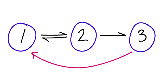
If a steady state is accessible, a system will tend to relax to it. (If external conditions are changing in time, then a steady state might not be accessible – but we won’t go there.) Since equilibrium is a steady state, relaxation could be to equilibrium or to a NESS. It will depend on how the system is set up – the ‘boundary conditions’. We are studying a NESS with a source and sink as boundary conditions. Here’s the sketch.
Here are the questions from last time.
-
Write down the exact solution to the set of ODEs. No math is required at all. Instead, use the solutions you already know for the two-state system, and just substitute in the rates.
-
Defining
 , we have
(1)
![\begin{align*} P_1(t) &= P^{ss}_1 + \left[ P_1(0) - P^{ss}_1 \right] e^{-q\, t} \nonumber \\ P_2(t) &= P^{ss}_2 + \left[ P_2(0) - P^{ss}_2 \right] e^{-q\, t} \nonumber \\ P_3(t) &= P^{ss}_3 = 0 \end{align*}](https://statisticalbiophysicsblog.org/wp-content/ql-cache/quicklatex.com-c9e51d87e91a4151494a18b3aeb0ee57_l3.png "Rendered by QuickLaTeX.com")
The
 values will be given below. These equations describe relaxation to the source-sink NESS with state 1 as the source and state 3 as the sink. (You may have caught my typo for these expressions on Physical Lens. I need to fix that!)
-
Defining
-
What is the new relaxation time (time constant of the exponential)? Does the (algebraic) dependence of this timescale on the various rate constants make sense?
-
The relaxation time constant is
 . Note that
  depends on all the rates, as we now should expect. But also it depends on all the rates in the same way – i.e., every transition equally affects the relaxation time. Interestingly, the overall rate will be large (fast) if any of the three component rates is large, but will only be small (slow) if all of the rates are small. The behavior of can be compared to the more complicated eigenvalues for the full system, as discussed on Physical Lens, but instead we will focus later on comparing to a related timescale, the mean first-passage time. Does the behavior of make sense? Well, more or less, we can say.
-
The relaxation time constant is
-
As
 , the system does not relax to equilibrium. Find the state probabilities and show that detailed balance does not hold – at least in the usual sense. That is, show that
  .
.
-
Using the notation
 , and setting time derivatives in the ODEs to zero, we find
(2)

where
 is the sum of the numerators to ensure normalization. To check detailed balance, we see that
-
Using the notation
-
Instead the system relaxes to a non-equilibrium steady state. Describe in words the basic property of any steady state and show that the steady probabilities satisfy this property for both states.
-
In steady state, the total flow into a state must match the total flow out. For state 2, this condition amounts to
 , which holds after substituting the values given above.
-
In steady state, the total flow into a state must match the total flow out. For state 2, this condition amounts to
-
Remind yourself that equilibrium [defined by detailed balance] is a special steady state. Explain why detailed balance implies steady state, but note that our system shows the reverse is not true in general.
-
If detailed balance holds, then for a given state
 , the flow into from any state
  will balance the flow out to from , so the summed flows (for
  ) must balance. Besides our system, a simple counter-example is a “triangular” system of three states with only unidirectional flows
  which can be in steady state but does not satisfy detailed balance.
-
If detailed balance holds, then for a given state
Here are the last questions on the three-state model. You’re getting close to your non-equilibrium certification!!
- Study the Hill relation, and be prepared to explain it to an undergraduate student.
- Use the Hill relation to calculate MFPT from state 1 to 3 for our linear 3-state system.
-
Compare the MFPT to , which is the time to relax to steady state.
- Summarize the key lessons learned from two and three-state systems.