
I think of knowledge like a house: it’s assembled from bricks that separately don’t do much. On its own, each brick is more prone to weathering. Likewise, each of our calculation bricks is easy to forget. We must learn to put these in context. We must always seek the connections to build a stronger house, which automatically preserves our individual bricks.
Sorry for the sanctimony, but hey, the future of your brain is at stake!
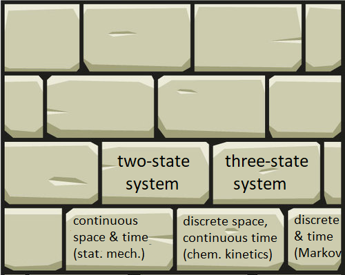
We have been looking at the simplest examples of discrete-state continuous-time systems ( not
not  ). We started there because the systems are simple and the ODE descriptions are familiar. Arguably the two-state and three-state systems each are bricks that we have cemented together.
But what about other types of theory? How do these systems relate to more fundamental statistical mechanics using continuous coordinates? And how does the continuous time get converted to the discrete-time descriptions we see so often Markov state models? You are going teach yourself these things.
We have been studying a non-equilibrium steady state (NESS) with a source and sink as boundary conditions.

Here are the questions from last time. If you have not actually done these with paper and pencil STOP HERE NOW. Do them or you’re wasting your time.
-
Study the Hill relation, and be prepared to explain it to an undergraduate student.
- When you meet me, I’m going to ask, so be ready.
-
Use the Hill relation to calculate the MFPT from state 1 to 3 for our linear 3-state system.
-
For the MFPT, we need the inverse flux. In steady state, the net flux from state 1 to 2 will be the same as from 2 to 3. For simplicity, we take the flux from 2 to 3:
 , with
  .
.
-
For the MFPT, we need the inverse flux. In steady state, the net flux from state 1 to 2 will be the same as from 2 to 3. For simplicity, we take the flux from 2 to 3:
-
Compare the MFPT to
 , which is the time to relax to steady state.
-
We wish to compare the MFPT,
 , to the relaxation time, . To do so, multiply both by
  and see that
  (proportional to MFPT) not only includes twice
  (proportional to NESS relaxation time) but it contains other strictly positive terms besides. (All rate constants are positive.) Hence the MFPT is expected be significantly longer than the relaxation time to NESS. Note that the three-state system is not fully representative of more complex systems in that any fast rate will make
  large and the relaxation to NESS very fast. More generally, you should expect that relaxation to a NESS will not be fast – just faster than relaxation to equilibrium.
-
We wish to compare the MFPT,
-
Summarize the key lessons learned from two and three-state systems.
- So many things to choose from! All of the following should make sense to you now: ● Systems tend to relax to steady states. ● Equilibrium is a special steady state satisfying detailed balance but many steady states are not in equilibrium. ● Although I didn’t emphasize it above, in a source-sink NESS, probabilities nearer the target tend to be smaller than the corresponding equilibrium values because the sink is like a vacuum cleaner perpetually sucking in probability. ● The Hill relation shows the inverse MFPT is given by the flux in a source-sink NESS. ● Relaxation times will depend on all the rate constants involved. ● For a non-equilibrium steady state, some of the rate constants may be removed from the relaxation time and make it much faster than the corresponding MFPT. Although we didn’t show it directly, you might guess that relaxation to NESS is faster than to equilibrium for the three-state system, which is shown here. ● Likewise, more complicated systems are described by more complicated equations including multiple exponentials.

In the next set of questions, we’ll focus on connecting to traditional continuous-space statistical mechanics. See the one-dimensional potential energy diagram above. You can look at a textbook (Ch. 4 of my paper book, for example) and also get some help here.
-
Draw a discrete free energy-level diagram corresponding to the continuous two state (A,B) system sketched above. Your diagram should consist of three free energy levels (A, B, barrier). Write down the Arrhenius expressions (in which the rate constant is proportional to the Boltzmann factor of the free-energy barrier height) in both directions. If the conformational free energy
 is defined according to
  , show that using Arrhenius-like rate constants causes detailed-balance to be satisfied.
 - What reasonable explanation can be given for the Arrhenius rate expression in terms of continuous-space equilibrium-ish statistical mechanics? And why should entropy differences enter the expression based on a one-dimensional picture?
- Describe a procedure by which you could computationally estimate the rate constants of a continuous two-state system by running trajectories.