I want to introduce machine learning (ML) to people outside the field, both non-mathematical scientists totally new to machine learning and quantitative folks who are novices. My qualifications for this are that I’m an outsider to ML myself, maybe an “advanced beginner” – with several years of experience. As I have learned ML, I try to keep an eye out for what’s important and what isn’t.
One thing that’s definitely not important for beginners is the equations, so we will keep those to a minimum.
Jargon is a bit of a different story, as we need to be comfortable interpreting and potentially designing ML studies. So we want to embrace the essential jargon, but of course with clear definitions. We want to train ourselves not to be intimidated by the jargon.
What is machine learning?
Let’s start with the most obvious jargon, ML itself. The ‘machine’ of course is just the computer and ‘learning’ is a stretch term. Computers themselves know nothing, even if it seems they do, especially in the artificial intelligence era. Computers only follow instructions, i.e., computer programs or code.
Put the M and L together and we merely mean a computer program that takes in a data and fits some parameters (numerical constants optimized for the data) of a “model.” In ML, a model is just the set of equations chosen by the person doing the programming.
Let’s make it concrete. It’s a good idea to construct a simple example in your mind, or on paper, or a computer if that’s natural for you. There’s little chance to learn a new and complicated thing in the abstract.

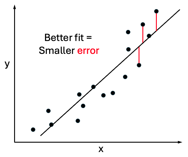
The simplest example is linear fitting, as shown in the figure. For now, this just means fitting a line through points, as you’ve likely seen before. It’s the simplest form of machine ‘learning’ because you can use the equation of the line to predict a y value for any new x value you’re given.
It’s the ability to make a prediction, based on learning (aka training) from data that makes it ML. Simple as pie.
For example, imagine we want to understand the relationship between the length and weight of a certain species of turtle, based on a whole bunch of measurements of each quantity (from a whole bunch of turtles). We can choose to treat the length as our single ‘independent variable’ and so for each turtle, the length will be the x value and the weight will be the y value, i.e., dependent variable. In a scatter plot of (x, y) points, each point would represent one turtle. Always keep track of what each point in a figure represents.
In ML we build models for our dependent variable(s) – what we want to be able to predict – based on the chosen dependent variables, also called features.
This is called supervised ML because we are using known y values (e.g., turtle weights) to train the parameters of the model. For now, we will focus only on supervised ML. For reference, unsupervised ML typically involves clustering data into groups or something similar.
Thus far, we have been talking about one-dimensional (1D) data, by which we mean just a bunch of numbers as x values, as opposed to vectors. A higher dimensional model for the weight of a turtle could build a model based on more than one ‘feature,’ say the length and height of the shell. Visualizing this data would require a three-dimensional plot, but we don’t need to pursue that now.
It’s also useful to know that any kind of data fitting based on continuous x and y values is called regression.
How does machine learning work?
Supervised machine learning is just fitting data, such as the linear model we just described.
The linear model assumes that y is simply a multiple of x, possibly with an additive constant: , where a and b are the parameters of the model.
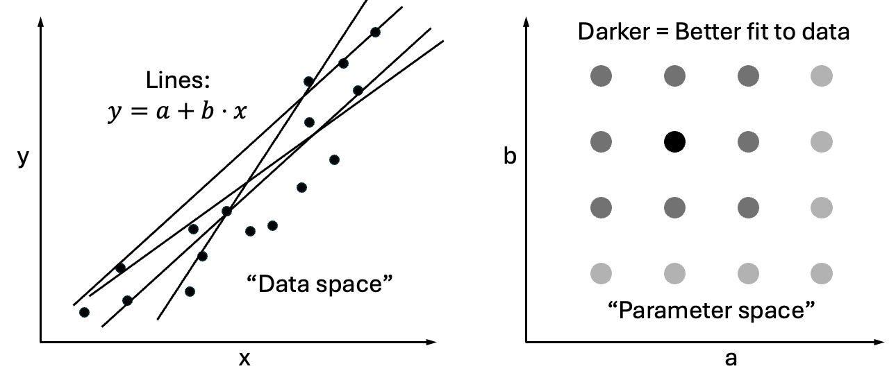
The essence of the process is not hard to understand. We can simply try every possible combination of the a and b parameters, and then choose the pair that gives the best fit.

This procedure would be a grid search because we are effectively creating a plane with a and b as axes (instead of x and y), upon which we can place a grid of evenly spaced values, i.e., (a, b) pairs, to try. This new plane is sometimes called a parameter space to distinguish it from the space of (x, y) data values.
How do we evaluate each pair of (a, b) values? We do so using a loss function which is a mathematical expression that quantifies our idea of goodness of fit. (I stress the word idea because one can invent different loss functions for different purposes, and this is a key but little discussed point for more advanced practitioners. I hope to return to this point in a future post.)
The most common loss function measures the average squared (vertical) distance of points from the line. That is, for every point, draw a vertical line up or down to the candidate fit line – which is based on candidate (a, b) values – and measure that distance, then square it, and average over all such distances. See red lines in the first figure, above.
In sum, machine learning for this case means writing a computer program to evaluate the loss function for every (a, b) pair of values on the grid, and assigning the minimum “loss” as the best fit. Then for any new value of x, the function with the best (a, b) values yields a prediction for y.
If you understand that, consider yourself a machine learner!
Say it in jargon: Optimization in parameter space
We already mentioned the plane of (a, b) values as a parameter space. By doing a grid search over this space – to find the best (a, b) pair which minimizes our choice of loss function – we are performing what’s called an optimization. No big deal, it’s just finding the smallest value.
What model should I use?
We have illustrated the essentials of machine learning by a linear fit. But there’s no rule of science that fits have to be linear. In the case of turtles, we would not expect the weight to vary linearly with length, but rather with a higher power of length. (A naïve guess would be the 3rd power, because weight should be proportional to volume, which in turn should vary with the cube of the linear dimension.)
You could imagine trying more complicated models, such as . These more complicated models are certain to fit the data as well or better than the simpler model. This is true even if the underlying process actually was linear because, with noise, the data won’t come out perfectly on a line, and thus the more complicated quadratic function is almost certain to provide a better fit.
But a better fit to the training data is not always desirable, as we’ll discuss.
The overfitting problem and test/validation data

The overfitting issue, in my view, is the single most important thing to know about machine learning. It teaches us about the limitations of ML, but also points the way toward improving models.
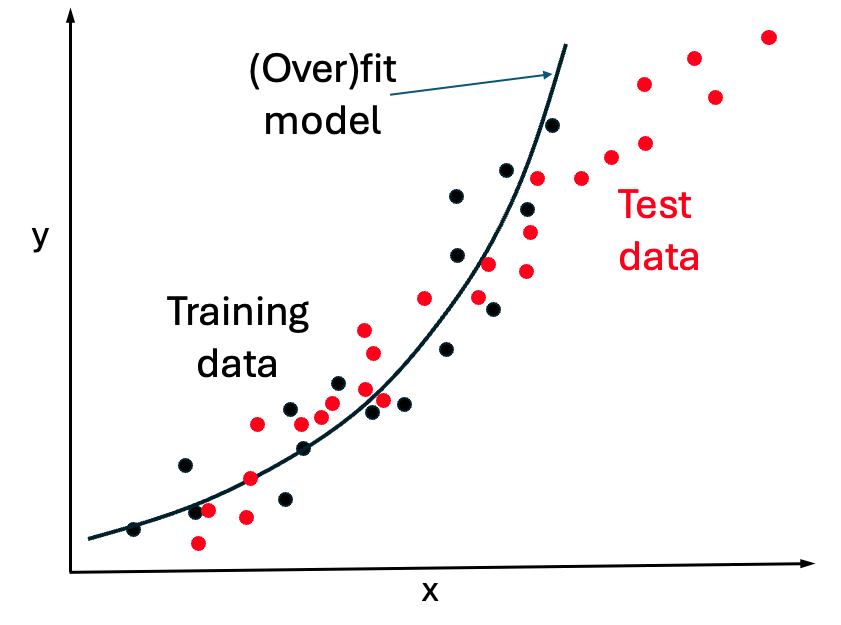
When we build a machine learning model, such as for the weight of turtles based on their length, the data used to fit the parameters is called the training data. It is critical to appreciate that the quality of the model cannot be evaluated based on the quality of the fit to the training data. Even if there is zero error in the fit, the model could be terrible in the sense of not being predictive for new data.
A ML model must be evaluated on set of test data (sometimes called validation data, although we won’t go into the nuances here) which has not been used in the training of the model. That is, the test data must not have been used to fit the parameters, such as a and b in the linear example.
The figure above (which is made up and not for turtles) suggests that a quadratic model was used to fit the training data in black, while the red test data suggests the trend is actually linear. Thus the black curve overfits the training data because it poorly describes independent data from the same system.
Overfitting describes the situation where an overly complex model was used to fit the training data such that the model is poor fit to new, test data.
Hence, any time you see a machine learning study, make sure you check that suitable, independent testing data was used. We will discuss some nuances of validation in a future post.
Summary
Supervised ML, known as regression for continuous variables (regular numbers) entails fitting parameters, namely, the constants for the equations which are chosen by the practitioner. Parameters are chosen that minimize the error in the fit. Testing on independent data is essential to check for overfitting. If the model does not provide a good fit for the test data, it’s likely a simpler model should be used. A future post will explore the important issue of constructing simple enough models.
It may seem ironic that I am emphasizing the importance of simpler models in the era of deep neural networks and artificial intelligence. The fact is that doing good science with ML requires “right-sized” models, not necessarily the model with the most intimidating name. Stay tuned.

