

The trajectory ensemble is everything you’ve always wanted, and more. Really, it is. Trajectory ensembles unlock fundamental ideas in statistical mechanics, including connections between equilibrium and non-equilibrium phenomena. Simple sketches of these objects immediately yield important equations without a lot of math. Give me the trajectory-ensemble pictures over fancy formalism any day. It’s harder to make a mistake with a picture than a complicated equation.
A trajectory, speaking roughly, is a time-ordered sequence of system configurations. Those configurations could be coordinates of atoms in a single molecule, the coordinates of many molecules, or whatever objects you like. We assume the sequence was generated by some real physical process, so typically we’re considering finite-temperature dynamics (which are intrinsically stochastic due to “unknowable” collisions with the thermal bath). The ‘time-ordered sequence’ of configurations really reflects continuous dynamics, so that the time-spacing between configurations is vanishingly small, but that won’t be important for this discussion.
A trajectory ensemble is a collection of such trajectories distributed according to some condition, which might be equilibrium or not.
The equilibrium trajectory ensemble is the best place to start. We’ll “make” this ensemble – in an old-fashioned thought-experiment way – by observing a large number of systems over a very long time. (You may imagine actual systems or computer simulations – it doesn’t matter.) Regardless of how we started the systems, after enough time they will become fully decorrelated from one another, and we will have an equilibrium ensemble on our hands.

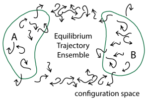
In the figure, each arrow schematically represents one trajectory. Importantly, this is NOT a picture of atoms or particles interacting, but a schematic view of many fully independent systems projected onto a single copy of the configuration space. The arrow tip represents the present configuration and the (curved) arrow shaft shows some recent history of the trajectory.
What can we learn from the equilibrium trajectory ensemble? In fact, anything we want to know about our system, but let’s start with equilibrium quantities of interest, a.k.a. equilibrium “observables”. Most prominently, if we take a fixed-time snapshot of the ensemble, such as all the configurations at the arrow tips, we have an equilibrium ensemble of configurations. That is, these configurations (x) will be distributed according to the Boltzmann factor, e^[-U(x)/kT] of the potential energy U if the systems live at temperature T. The equilibrium distribution of configurations is obtained from trajectories because dynamics are the ultimate source of equilibrium behavior: nature directly “encodes” only dynamics – we humans infer thermodynamics (e.g., equilibrium). Put another way, no molecule “knows” how it should participate in an ensemble or distribution; a molecule can only blindly behave according to the forces it feels.
With the equilibrium distribution of configurations in hand, we can calculate any equilibrium quantity we like. We can calculate the average of any observable … just by averaging the observable over the ensemble. We can obtain the potential of mean force along an arbitrary coordinate by histogramming our ensemble along that coordinate and taking a log. The free energy difference between any two configurational states (e.g., A and B in the figure below) can be obtained by taking the log of the ratio of counts of arrow tips in each state.
So what’s different and special about the ensemble of trajectories, compared to the “mere” ensemble of configurations? Trajectories also tell us about dynamical processes – their rates and mechanisms.
From a trajectory ensemble, we can infer a “mechanism” for a process … but we cannot from a configurational ensemble. Assume we’re interested in transitions from state A to B in the figure. Perhaps A is the closed state of an enzyme and B is the open state. The mechanism may then be defined as the weighted set of pathways taken from A to B – e.g., the fraction of trajectories taking the lower vs the upper pathway in the figure. Physically these might correspond to different orderings of events, such as which sub-domain of the enzyme opens first. (The enzyme adenylate kinase provides a good illustration of the potential for path heterogeneity.)
When we think about mechanism in the trajectory-ensemble picture, we see that some conventional conceptions of mechanism are inadequate for complex systems. For example, the notion of a single transition state or even a ‘transition state ensemble’ (e.g., of configurations as likely to reach A before B as the reverse) do not describe the sequence possible intermediates through which a complex system may pass, let alone the possible multiplicity of pathways. Our picture, in the literal sense, makes all this clear.
Can kinetic information – rate constants – be obtained from an equilibrium ensemble of trajectories? Yes, because trajectories are intrinsically dynamical. The trick is to examine a suitable subset of trajectories.
In a previous post, we saw that the rate (expressed as the inverse of the mean first-passage time, MFPT) could be obtained from a steady-state ensemble of trajectories. This is because, according to the Hill relation, the fraction of trajectories arriving to B from A per unit time in a steady state is exactly the inverse MFPT.
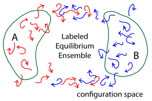
To obtain a steady-state ensemble of trajectories transitioning from A to B – which in turn will yield the MFPT – we can use a labeling idea developed by vanden Eijnden and others (as re-formulated in Bhatt & Zuckerman, 2011) to select out a subset of the equilibrium trajectory ensemble that corresponds precisely to an A-to-B steady state. Quite simply, we label (or color red, in the figure) all trajectories which were more recently in A in than B. This labeling exactly dissects the equilibrium ensemble into the A-to-B and B-to-A steady-states. (Because our trajectory ensemble is in equilibrium, the same number of red trajectories will turn blue – on entering B – as will turn red per unit time, on average.)
From that red-colored A-to-B steady state, we can get the MFPT (inverse rate) using the Hill relation.
In summary … we can see the power of trajectory thinking. Concepts are clarified, equations justified, and calculational approaches engendered.
From the equilibrium trajectory ensemble, it’s straightforward to obtain equilibrium observables, and kinetic quantities can be estimated from suitable subsets of the full ensemble.
Before we finish, it’s worth discussing when a single trajectory might provide the same information as the equilibrium trajectory ensemble. This would hold only for a truly long trajectory – one in which all important transitions have been seen multiple times. (One could obtain the equilibrium ensemble from a set of points on the trajectory, for example.) Anything shorter might be called an ‘equilibrium trajectory’, but that name only reflects a lack of external driving forces, not the utility for calculating valid observables.
References
“Zipping and unzipping of adenylate kinase: atomistic insights into the ensemble of open-closed transitions,” Beckstein, O.; Denning, E. J.; Perilla, J. R. & Woolf, T. B. J Mol Biol, 2009, 394, 160-176
“Heterogeneous Path Ensembles for Conformational Transitions in Semiatomistic Models of Adenylate Kinase,” Bhatt, D. & Zuckerman, D. M. Journal of Chemical Theory and Computation, 2010, 6, 3527-3539
“Beyond Microscopic Reversibility: Are Observable Nonequilibrium Processes Precisely Reversible?,” Bhatt, D. & Zuckerman, D. M., Journal of Chemical Theory and Computation, 2011, 7, 2520-2527
“Separating forward and backward pathways in nonequilibrium umbrella sampling,” Dickson, A.; Warmflash, A. & Dinner, A. R., J Chem Phys, 2009, 131, 154104
“A novel path sampling method for the calculation of rate constants,” van Erp, T. S.; Moroni, D. & Bolhuis, P. G., The Journal of chemical physics, 2003, 118, 7762-7774
“Exact rate calculations by trajectory parallelization and tilting,” Vanden-Eijnden, E. & Venturoli, M., J Chem Phys, 2009, 131, 044120
Statistical Physics of Biomolecules: An Introduction, Zuckerman, D. M., CRC Press, 2010