The “Hill relation” is a key result for anyone interested in calculating rates from trajectories of any kind, whether molecular simulations or otherwise. I am not aware of any really clear explanation, including Hill’s original presentation. Hopefully this go-around will make sense.
The Hill relation applies to any “first passage” process – which could be diffusion from one region to another, chemical isomerization, protein folding, a cell-signaling process, or …. Quite simply, a first-passage process is one in which a system is initialized somehow (it doesn’t matter how but the initialization should be well-specified or at least reproducible) and a hypothetical observer waits until a target state is reached or occurs (any target state will do). The observer could measure the time required for each occurrence, and the average time for such a process is called mean first passage time (MFPT). The inverse MFPT is one common definition for a rate constant, because the MFPT clearly describes the timescale for the process.
The Hill relation tells us that in a steady state (SS) implementation of a first-passage process – where trajectories are initiated from some arbitrary state A and terminated upon reaching another, separate state B (at which time they are re-initiated at A) – that the inverse of the mean first-passage time (1/MFPT) is given exactly by the probability flux into B, i.e., the fraction of trajectories entering state B per second.
= Fraction of trajectories which started in A that arrive to B in steady state per unit time
We assume that trajectories are initiated according to some desired distribution from state A. (Different distributions of initial phase-space points will lead to different MFPTs, not surprisingly. We’re just going to assume you’re happy with some initial distribution, though it’s worth noting that the choice of initial distribution requires a more subtle discussion: see the paper by Bhatt and Zuckerman.)
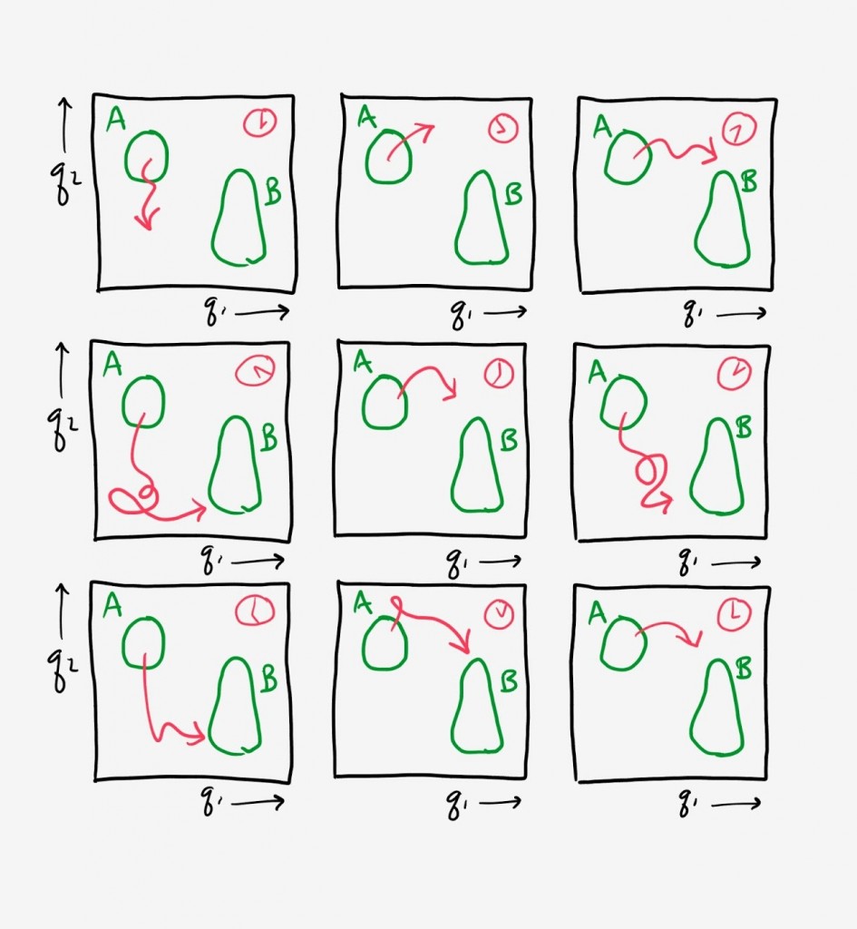
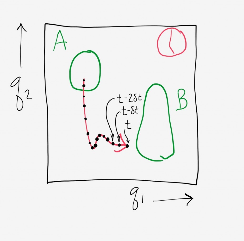
To derive the relation, we will imagine running a very large number of fully independent simulations for a very long time. The schematic shows a set of red trajectories projected onto two coordinates. Importantly, we record the full history of each trajectory – the coordinates at all times – and we see a large number of A-to-B transitions.
Because we have all information about the trajectories in the steady state, we can go back and examine precisely where each was at all times in the past. This enables us to perform the simple transformation of “stretching” out each trajectory in such a way that we examine it in terms of its temporal progress toward state B. This is like waiting at a bus stop with your smart phone and seeing the future arrival times of all the buses, regardless of the bus route.
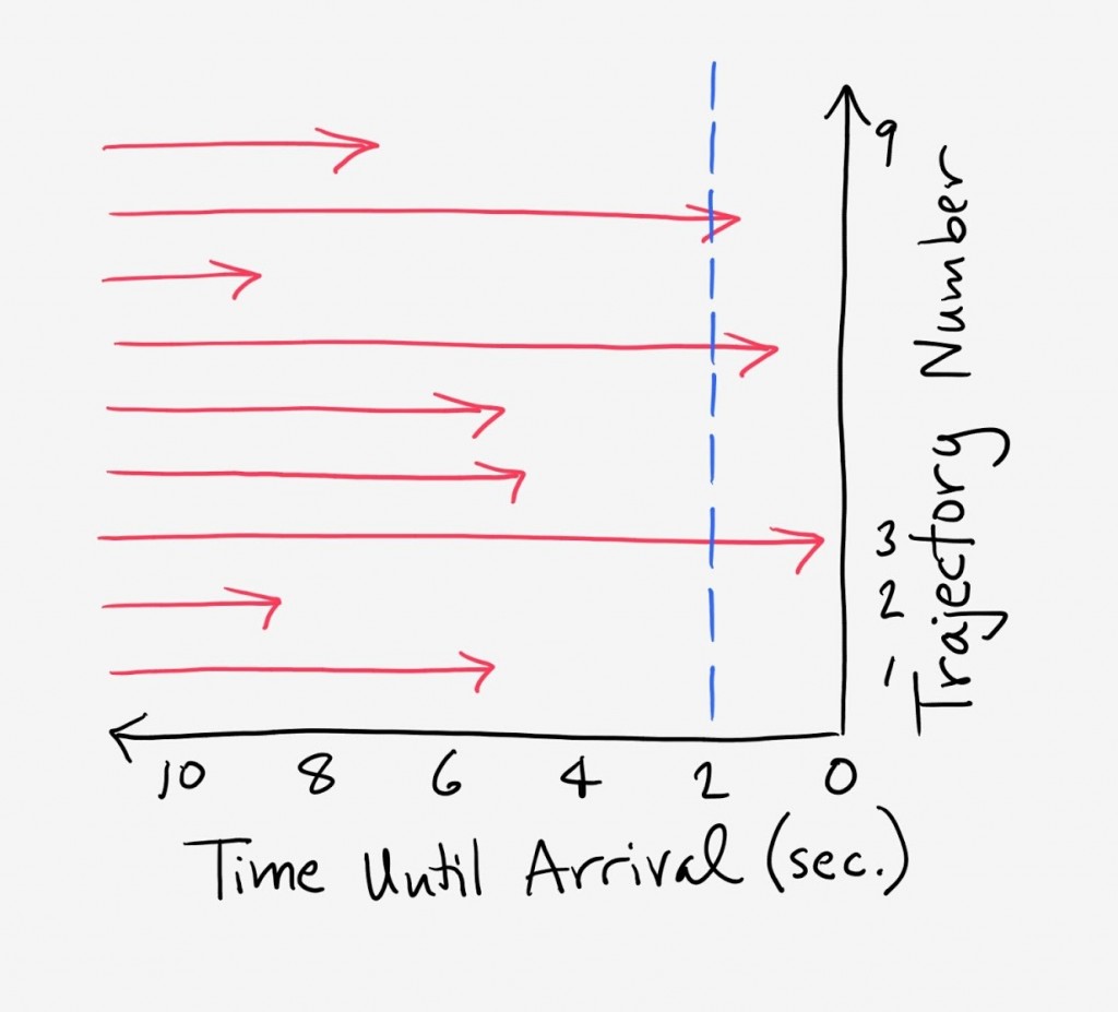
Hence we develop a picture like that shown below, with each red trajectory marching toward its arrival in state B. We know how long each trajectory will take to arrive because we (imagine we) have simulated each long into the past and future.
We can calculate the probability flux into state B in two ways that must be equivalent. First, because our independent trajectories have been running for a very long time, we assume they have become fully decorrelated. Hence we expect that in any interval of time, the same fraction of trajectories will arrive to state B. In the figure, we see that 3 trajectories will arrive in the next two seconds. Equivalently, ⅓ of the trajectories will arrive in 2 seconds, so that the probability flux is ⅙ per second.
We also expect that, because the trajectories are fully independent and de-correlated, in any time interval Δt, the fraction of trajectories arriving should be Δt/MFPT. After all, the MFPT is the average time a trajectory should spend in transit, so our chance to observe it in time Δt should be Δt/MFPT on average. (If you want to think about this more concretely, imagine restarting a single trajectory from A each time it arrives to B, creating a sequence of first-passage events. The average of the first-passage times will be the MFPT, by definition, and so the probability to observe an event will Δt/MFPT.) In the example shown, we expect a fraction (2 sec)/MFPT of the trajectories to arrive in the 2 sec time interval. When the MFPT is 6 seconds, then ⅓ of the trajectories should arrive in 2 sec. Conversely, if we see that ⅓ of the trajectories arrive in 2 sec, we know the MFPT = 6 sec.
Thus we have it: Probability Flux = 1/MFPT. Importantly, this is an exact result, not dependent on the type of dynamics or any assumptions about the states or the initial distribution (of starting points).
The reason I consider the Hill relation a “remarkable result,” even if it gets to seem obvious when you think about it for too long, is that provides a means in principle for calculating a very long timescale (the MFPT) from an arbitrarily short observation period (of a steady-state ensemble of trajectories). Although generating a steady-state ensemble in a naive way would require times of the same order as the MFPT itself, there are specialized methods that permit the indirect inference of steady-state information from short simulations. These are path-sampling methods including the weighted ensemble approach, milestoning, transition interface sampling, forward flux sampling, non-equilibrium umbrella sampling and others.
The Hill relation also exemplifies the power of using the trajectory-ensemble picture. With a minimum of equations, the trajectory-ensemble view of statistical mechanics permits the development of powerful results and calculational methods. Stay tuned for more.
References
- Terrell L. Hill, Free Energy Transduction and Biochemical Cycle Kinetics (Dover, 2004)
- “Beyond microscopic reversibility: Are observable non-equilibrium processes precisely reversible?”, Divesh Bhatt and Daniel M. Zuckerman, Chem. Theory Comp., 7:2520-2527 (2011).


