
Trajectories are golden information in the study of dynamical systems like cells. If we can follow individual cells in time, then we can learn what events precede others and in principle infer all kinds of wonderful mechanistic information.
The problem is that measurements that reveal high-dimensional omics information for single cells require killing the cells, whereas observing cells in real time via video microscopy doesn’t reveal too much molecular information. Although modern live-cell microscopy techniques enable labeling specific cellular proteins to reveal their spatial and temporal intra-cellular behavior, this is limited to a literal handful of proteins (at once). And there’s always the worry that the labels may alter the behavior of cells.
So the question is, How can we learn detailed information for single cells as they change and move in time? In other words, can we learn about (apparently) hidden information?
A big part of the answer, in my mind, is delay embedding — a highly intuitive approach with a firm mathematical basis. Originally developed as part of dynamical systems theory, the approach has applications in many fields of science. There is a beautiful review article covering the subject which I highly recommend.
The essence of delay embedding can be understood by thinking about a ball. Delay embedding involves analyzing a temporal sequence of observations (in order).
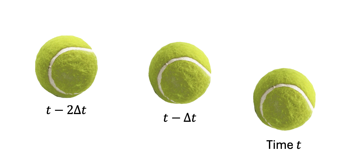
You don’t need a Ph.D. in physics to understand key aspects of this example: (i) if you see just one snapshot in time of a ball, you don’t know which way it’s moving; (ii) if you see a second snapshot, you can estimate the velocity of the ball – both translational and rotational components; (iii) if you see a third snapshot, you can estimate how those velocities are changing in time.
By seeing a time-sequence of images, you can learn about coordinates which cannot be measured via a single snapshot, namely velocity and acceleration. And it’s interesting to note that some of the acceleration is due to the environment (air resistance) so in fact, you can learn about coordinates that are not directly part of the object itself. These are truly hidden coordinates that are revealed by delay embedding.
In fact, the seminal theorem of delay embedding tells us that for a deterministic system, there is a mapping (albeit unknown) between every coordinate of the system and the “vector” formed by concatenating a sufficiently long time sequence of observations (e.g., on a subset of coordinates).
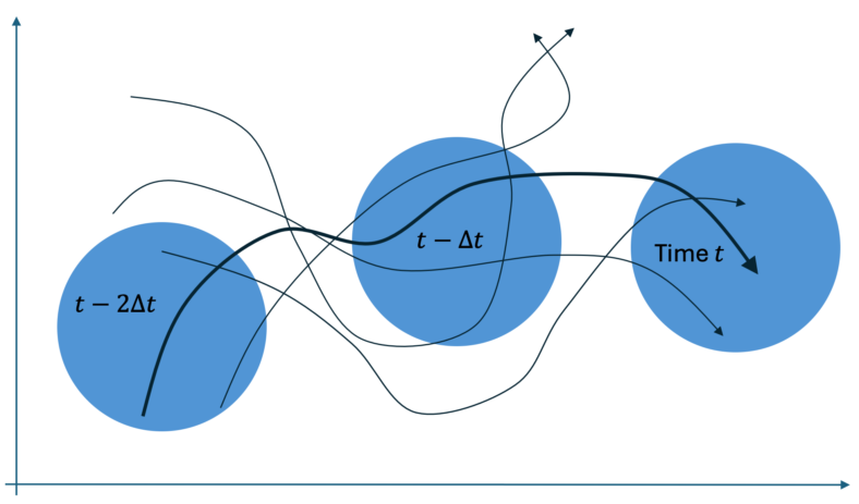
Let’s see how the basic idea might work for cells, based on the cartoon figure below. Each black trajectory represents possible single-cell behavior over time, projected into a two-dimensional space of measurable quantities. If we assume that each cell evolves deterministically based on its initial conditions, we are trying to determine which cell (which trajectory) was observed in a particular sequence of measurements. (The question of deterministic vs. stochastic behavior was addressed in a previous post.)
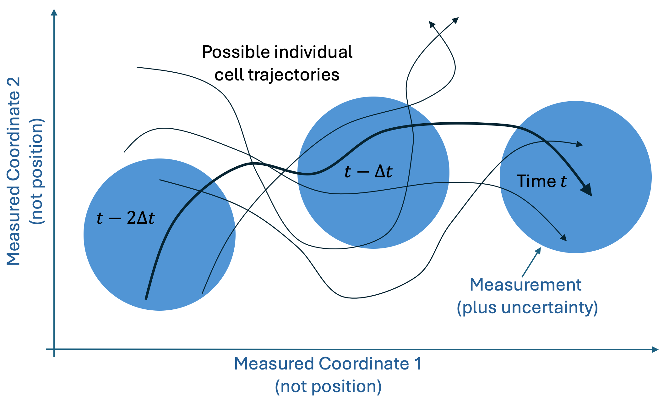
We imagine measuring only two “coordinates” of a cell (e.g., the cell area and the ratio of short to long axis) and with some uncertainty, represented by the blue circles. Importantly, the blue circles are not position coordinates, so for any given measurement (within one blue circle) there are numerous single-cell trajectories consistent with that measurement. However, as we include more measurements (blue circles) we increasingly narrow down the number of trajectories consistent with that sequence of measurements – ideally until we narrow it down to a unique trajectory (think black curve).
This is amazing. Delay embedding truly reveals hidden information. In the limit of enough data, it should yield a description equivalent to the “microscopic state” of a cell consisting of all molecular species, etc.
But delay embedding on its own is not a complete solution to cell behavior. After all, using the procedure I just described, we only end up with a time-ordered list of features. We may assert that list is equivalent to a cell’s microscopic state, but we don’t directly learn the molecular features of interest – e.g., protein expression levels and spatial distributions.
To learn biology, we have to develop a mapping from the delay-embedded vectors of observables to the biological features of interest, and machine learning is the natural way to do this. What’s called for is, in principle, fairly standard: if we can obtain matched pairs of delay-embedded trajectories and molecular quantities of interest, we can perform ordinary regression.
So the practical question is whether we can do this kind of machine learning. The answer, I say, is yes, and you can get a glimpse of our approach in this preprint. Stay tuned for more.