Category: Trajectory physics/analysis

Caution Regarding Markov State Models

Markov state models (MSMs) are very popular and have a rigorous basis in principle, but applying them in practice must be done with great caution. There is no guarantee the results will be reliable for complex systems of typical interest unless there is an enormous amount of data and significant expertise and validation goes into the MSM building. And even if those conditions are in place, certain observables likely will be biased.
Continue reading

A “proof” of the discretized Hill Relation

This is yet another one of those things where, after reading this, you’re supposed to say, “Oh, that’s obvious.” And I admit it is kind of obvious … after you think about it for a few minutes! So spend those few minutes now to learn one more cool thing about non-equilibrium trajectory physics.

In non-equilibrium calculations of transition processes, we often wish to estimate a rate constant, which can be quantified as the inverse of the mean first-passage time (MFPT). That is, one way to define a rate constant is just reciprocal of the average time it takes for a transition. The Hill relation tells us that probability flow per second into a target state of interest (state “B”, defined by us) is exactly the inverse MFPT … so long as we measure that flow in the A-to-B steady state based on initializing trajectories outside state B according to some distribution (state “A”, defined by us) and we remove trajectories reaching state B and re-initialize them in A according to our chosen distribution.

Continue reading

Let’s stop being sloppy about uncertainty

Let’s draw a line. Across the calendar, I mean. Let’s all pledge that from today on we’re going to give honest accounting of the uncertainty in our data. I mean ‘honest’ in the sense that if someone tried to reproduce our data in the future, their confidence interval and ours would overlap.

There are a few conceptual issues to address up front. Let’s set up our discussion in terms of some variable q which we measure in a molecular dynamics (MD) simulation at successive configurations: q_0, q_1, q_2, and so on. Regardless of the length of our simulation, we can measure the average of all the values \overline{q}= \displaystyle\sum_{i=1}^{M} q_i. We can also calculate the standard deviation σ of these values in the usual way as the square root of the variance. Both of these quantities will approach their “true” values (based on the simulation protocol) with enough sampling – with large enough M.

Continue reading

What I have against (most) PMF calculations

Such a beautiful thing, the PMF. The potential of mean force is a ‘free energy landscape’ – the energy-like-function whose Boltzmann factor exp[ -PMF(x) / kT ] gives the relative probability* for any coordinate (or coordinate set) x by integrating out (averaging over) all other coordinates. For example, x could be the angle between two domains in a protein or the distance of a ligand from a binding site.

The PMF’s basis in statistical mechanics is clear. When visualized, its basins and barriers cry out “Mechanism!’’ and kinetics are often inferred from the heights of these features.

Yet aside from the probability part of the preceding paragraph, the rest is largely speculative and subjective … and that’s assuming the PMF is well-sampled, which I highly doubt in most biomolecular cases of interest.

Continue reading

So you want to do some path sampling…

Basic strategies, timescales, and limitations

Key biomolecular events – such as conformational changes, folding, and binding – that are challenging to study using straightforward simulation may be amenable to study using “path sampling” methods.  But there are a few things you should think about before getting started on path sampling.  There are fairly generic features and limitations that govern all the path sampling methods I’m aware of.

Path sampling refers to a large family of methods that, rather than having the goal of generating an ensemble of system configurations, attempt to generate an ensemble of dynamical trajectories.  Here we are talking about trajectory ensembles that are precisely defined in statistical mechanics.  As we have noted in another post, there are different kinds of trajectory ensembles – most importantly, the equilibrium ensemble, non-equilibrium steady states, and the initialized ensemble which will relax to steady state.  Typically, one wants to generate trajectories exhibiting events of interest – e.g., binding, folding, conformational change.

Continue reading

FAQ on Trajectory Ensembles

Q: What is a trajectory?

A trajectory is the time-ordered sequence of system configurations which occur as all the coordinates evolve in time following some rules – hopefully rules embodying reasonable physical dynamics, such as Newton’s laws or constant-temperature molecular dynamics.

Q: What is a trajectory ensemble?

It’s a set of independent trajectories that together characterize a particular condition such as equilibrium or a non-equilibrium steady state.  That is, the trajectories do not interact in any way, but statistically they describe some condition because of how they have been initiated – and when they are observed relative to their initialization … see below.

Continue reading

More is better: The trajectory ensemble picture

The trajectory ensemble is everything you’ve always wanted, and more.  Really, it is.  Trajectory ensembles unlock fundamental ideas in statistical mechanics, including connections between equilibrium and non-equilibrium phenomena.  Simple sketches of these objects immediately yield important equations without a lot of math.  Give me the trajectory-ensemble pictures over fancy formalism any day.  It’s harder to make a mistake with a picture than a complicated equation.

A trajectory, speaking roughly, is a time-ordered sequence of system configurations.  Those configurations could be coordinates of atoms in a single molecule, the coordinates of many molecules, or whatever objects you like.  We assume the sequence was generated by some real physical process, so typically we’re considering finite-temperature dynamics (which are intrinsically stochastic due to “unknowable” collisions with the thermal bath).  The ‘time-ordered sequence’ of configurations really reflects continuous dynamics, so that the time-spacing between configurations is vanishingly small, but that won’t be important for this discussion.

Continue reading

Everything is Markovian; nothing is Markovian

The Markov model, without question, is one of the most powerful and elegant tools available in many fields of biological modeling and beyond.  In my world of molecular simulation, Markov models have provided analyses more insightful than would be possible with direct simulation alone.  And I’m a user, too.  Markov models, in their chemical-kinetics guise, play a prominent role in illustrating cellular biophysics in my online book, Physical Lens on the Cell.

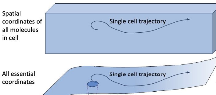
Yet it’s fair to say that everything is Markovian and nothing is Markovian – and we need to understand this.

If you’re new to the business, a quick word on what “Markovian” means.  A Markov process is a stochastic process where the future (i.e., the distribution of future outcomes) depends only on the present state of the system.  Good examples would be chemical kinetics models with transition probabilities governed by rate constants or simple Monte Carlo simulation (a.k.a. Markov-chain Monte Carlo).  To determine the next state of the system, we don’t care about the past: only the present state matters.

Continue reading